44 excel chart change labels

Create Dynamic Chart Data Labels with Slicers - Excel Campus Feb 10, 2016 · Typically a chart will display data labels based on the underlying source data for the chart. In Excel 2013 a new feature called “Value from Cells” was introduced. This feature allows us to specify the a range that we want to use for the labels. Since our data labels will change between a currency ($) and percentage (%) formats, we need a ... How to Use Cell Values for Excel Chart Labels Select the chart, choose the "Chart Elements" option, click the "Data Labels" arrow, and then "More Options." Uncheck the "Value" box and check the "Value From Cells" box. Select cells C2:C6 to use for the data label range and then click the "OK" button. The values from these cells are now used for the chart data labels.

Excel Chart Data Labels-Modifying Orientation - Microsoft ... Replied on September 14, 2016 In reply to PaulaAB's post on September 13, 2016 Hi Paula, You can right click on the data label part then select Format Axis. Click on the Size & Properties tab then adjust the Text Direction or Custom Angle. Thanks, Mike Report abuse 6 people found this reply helpful · Was this reply helpful? Replies (7)

Excel chart change labels

How to Customize Your Excel Pivot Chart Data Labels - dummies To add data labels, just select the command that corresponds to the location you want. To remove the labels, select the None command. If you want to specify what Excel should use for the data label, choose the More Data Labels Options command from the Data Labels menu. Excel displays the Format Data Labels pane. Add a DATA LABEL to ONE POINT on a chart in Excel | Excel ... Method — add one data label to a chart line Steps shown in the video above:. Click on the chart line to add the data point to. All the data points will be highlighted.; Click again on the single point that you want to add a data label to.; Right-click and select 'Add data label' This is the key step! How to edit the label of a chart in Excel? - Stack Overflow The latter box will list the "1", "2", etc. numbers that you want to change. Hit the edit button for the right-hand box (Horizontal Category (Axis) Labels), and you will be prompted to enter an axis label range. Instead of selecting a range, though, just enter the labels that you want to see on the x-axis, separated by commas, like so:

Excel chart change labels. Change axis labels in a chart in Office To change the label, you can change the text in the source data. If you don't want to change the text of the source data, you can create label text just for the chart you're working on. In addition to changing the text of labels, you can also change their appearance by adjusting formats. Edit titles or data labels in a chart The first click selects the data labels for the whole data series, and the second click selects the individual data label. Right-click the data label, and then click Format Data Label or Format Data Labels. Click Label Options if it's not selected, and then select the Reset Label Text check box. Top of Page Excel tutorial: How to customize axis labels Instead you'll need to open up the Select Data window. Here you'll see the horizontal axis labels listed on the right. Click the edit button to access the label range. It's not obvious, but you can type arbitrary labels separated with commas in this field. So I can just enter A through F. When I click OK, the chart is updated. Individually Formatted Category Axis Labels - Peltier Tech In the column chart, you need to change the chart type of the added column series to a line chart. Format the category axis (horizontal axis) so it has no labels. Add data labels to the the dummy series.

Insert a chart from an Excel spreadsheet into Word To update the chart automatically, change the data in the embedded workbook. Keep Source Formatting & Embed Workbook. Keeps the Excel theme. Embeds a copy of the Excel workbook with the chart. The chart doesn’t stay linked to the original workbook. To update the chart automatically, change the data in the embedded workbook. Excel Custom Chart Labels - My Online Training Hub Using Excel custom chart labels is a great way to create a more insightful chart without having to show a whole other series. Just take this chart below with custom labels showing the year on year % change: How to add or move data labels in Excel chart? In Excel 2013 or 2016. 1. Click the chart to show the Chart Elements button . 2. Then click the Chart Elements, and check Data Labels, then you can click the arrow to choose an option about the data labels in the sub menu. See screenshot: In Excel 2010 or 2007. 1. click on the chart to show the Layout tab in the Chart Tools group. See ... Excel charts: add title, customize chart axis, legend and ... How to change data displayed on labels To change what is displayed on the data labels in your chart, click the Chart Elements button > Data Labels > More options… This will bring up the Format Data Labels pane on the right of your worksheet. Switch to the Label Options tab, and select the option (s) you want under Label Contains:

How to rotate axis labels in chart in Excel? Go to the chart and right click its axis labels you will rotate, and select the Format Axis from the context menu. 2. In the Format Axis pane in the right, click the Size & Properties button, click the Text direction box, and specify one direction from the drop down list. See screen shot below: The Best Office Productivity Tools Add / Move Data Labels in Charts - Excel & Google Sheets ... Adding Data Labels Click on the graph Select + Sign in the top right of the graph Check Data Labels Change Position of Data Labels Click on the arrow next to Data Labels to change the position of where the labels are in relation to the bar chart Final Graph with Data Labels 2/ Right-click i.e. on the 1st histo. bar (A) > Add Data Labels (numbers are displayed a the top of the bars) 3/ Click one of the numbers that just displayed (the Format Data Labels pane opens on the right) > Check option "Value From Cells" > Select range C2:C7 > OK > Uncheck option "Value" demo.png (18.5 KiB) · 3 Remove Zero from Chart Data Labels #Shorts - YouTube #ExcelShorts #ExcelChartsHello Friends,In this video, you will learn how to remove zeros form chart data labels.Download our free Excel utility Tool and impr...

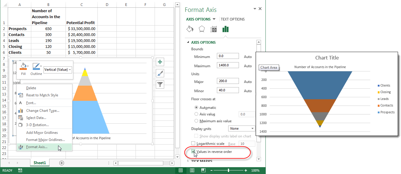
How to Create an Excel Funnel Chart | Pryor Learning Solutions

How to create Custom Data Labels in Excel Charts Create the chart as usual. Add default data labels. Click on each unwanted label (using slow double click) and delete it. Select each item where you want the custom label one at a time. Press F2 to move focus to the Formula editing box. Type the equal to sign. Now click on the cell which contains the appropriate label.

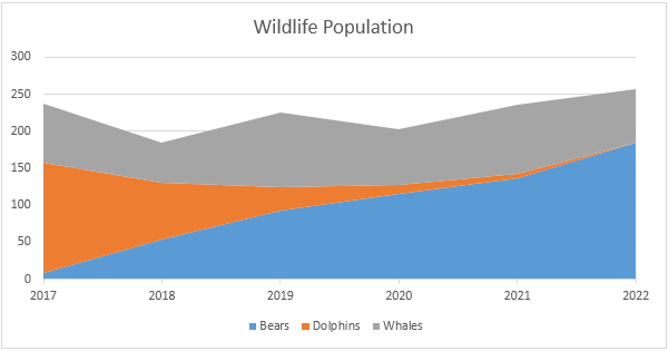
Area Chart in Excel - Easy Excel Tutorial

Custom Data Labels with Colors and Symbols in Excel Charts ... The chart will show the upward and downward arrow instantly. 1.1.1 Problems. Problem as I said in the beginning is that though the data labels I connected will update if data changes, but if I throw additional rows to the chart, the new data labels needs to be connected too and that makes it quite cumbersome.

Share :