42 excel scatter chart labels
TickLabels object (Excel) | Microsoft Docs To change the tick-mark label text for the value axis, you must change the values of these properties. Example. Use the TickLabels property of the Axis object to return the TickLabels object. The following example sets the number format for the tick-mark labels on the value axis in embedded chart one on Sheet1. Excel: How to Create a Bubble Chart with Labels - Statology Step 3: Add Labels. To add labels to the bubble chart, click anywhere on the chart and then click the green plus "+" sign in the top right corner. Then click the arrow next to Data Labels and then click More Options in the dropdown menu: In the panel that appears on the right side of the screen, check the box next to Value From Cells within ...
› pie-chart-in-excelPie Chart in Excel | How to Create Pie Chart | Step-by-Step ... Excel Pie Chart ( Table of Contents ) Pie Chart in Excel; How to Make Pie Chart in Excel? Pie Chart in Excel. Pie Chart in Excel is used for showing the completion or main contribution of different segments out of 100%. It is like each value represents the portion of the Slice from the total complete Pie. For Example, we have 4 values A, B, C ...
Excel scatter chart labels
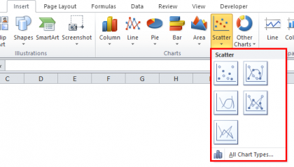
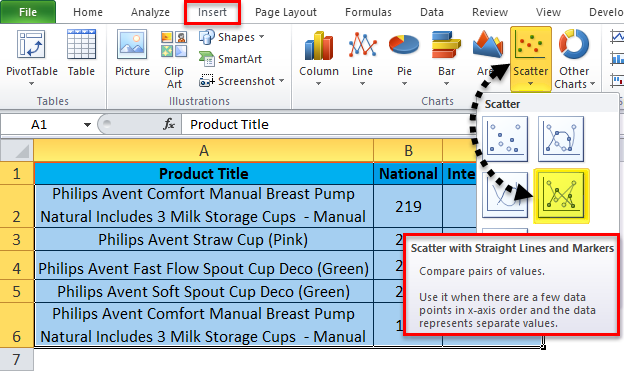
Quickly creating a x-y scatter chart with straight lines and markers ... Select the range. Insert a scatter chart with lines and markers. If it looks wrong, click anywhere in the chart. On the Chart Design tab of the ribbon, click Switch Row/Column. Here is an example. First, the scatter chart as created by Excel: Next, the result of clicking Switch Row/Column: Overlapping Circles on Scatter Chart overlaps labels My older version doesn't have the support for data labels that yours does, but here's what I did to approximate it: 1) Add two columns to the data table. 2) In column AG, enter Y values for positioning the data label. How to Find, Highlight, and Label a Data Point in Excel Scatter Plot ... By default, the data labels are the y-coordinates. Step 3: Right-click on any of the data labels. A drop-down appears. Click on the Format Data Labels… option. Step 4: Format Data Labels dialogue box appears. Under the Label Options, check the box Value from Cells . Step 5: Data Label Range dialogue-box appears.
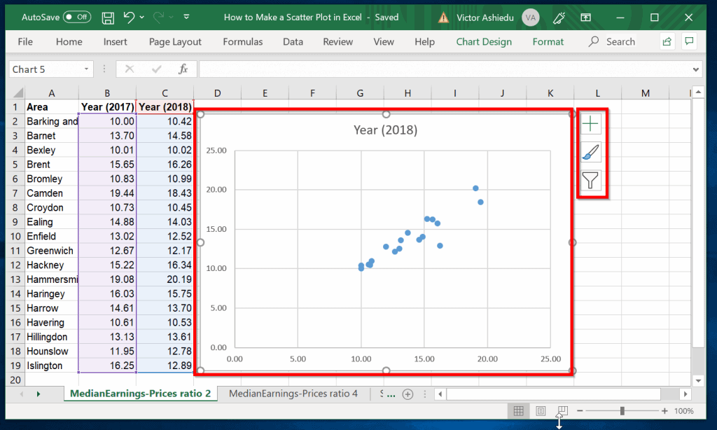
Excel scatter chart labels. › make-a-scatter-plot-in-excelHow to Make a Scatter Plot in Excel and Present Your Data - MUO May 17, 2021 · Add Labels to Scatter Plot Excel Data Points. You can label the data points in the X and Y chart in Microsoft Excel by following these steps: Click on any blank space of the chart and then select the Chart Elements (looks like a plus icon). Then select the Data Labels and click on the black arrow to open More Options. Label line chart series - Get Digital Help To label each line we need a cell range with the same size as the chart source data. Simply copy the chart source data range and paste it to your worksheet, then delete all data. All cells are now empty. Copy categories (Regions in this example) and paste to the last column (2018). Those correspond to the last data points in each series. XY Scatter Chart in Excel - Usage, Types, Scatter Chart - Excel Unlocked To add the Data Labels on the chart:- Click on the chart On the top right corner of chart, a + icon would appear. Click on it. Mark the Data Labels from the menu and click on More Options This opens the Format Data Labels Pane on the right of the excel window. From there mark the X and Y coordinates to be displayed via the Data Labels. Scatter, bubble, and dot plot charts in Power BI - Power BI Create a scatter chart. Start on a blank report page and from the Fields pane, select these fields:. Sales > Sales Per Sq Ft. Sales > Total Sales Variance %. District > District. In the Visualization pane, select to convert the cluster column chart to a scatter chart.. Drag District from Values to Legend.. Power BI displays a scatter chart that plots Total Sales Variance % along the Y-Axis ...
Guides: Data & Digital Scholarship Tutorials: Excel Scatter Plots Tutorial Procedures (1) Download Sample Data (2) Create Basic Scatter Plot (3) Style Chart (4) Direct v. Inverse (5) Regression Line (6) Dynamic Dropdown Menus Download the sample spreadsheet for this tutorial. This sample data contains the following columns: County [every county in the United States] State [state where the county resides] How to Apply a Filter to a Chart in Microsoft Excel - How-To Geek Go to the Home tab, click the Sort & Filter drop-down arrow in the ribbon, and choose "Filter.". Click the arrow at the top of the column for the chart data you want to filter. Use the Filter section of the pop-up box to filter by color, condition, or value. When you finish, click "Apply Filter" or check the box for Auto Apply to see ... › add-vertical-line-excel-chartAdd vertical line to Excel chart: scatter plot, bar and line ... May 15, 2019 · Add vertical line to Excel scatter chart; Insert vertical line in Excel bar chart; Add vertical line to line chart; How to add vertical line to scatter plot. To highlight an important data point in a scatter chart and clearly define its position on the x-axis (or both x and y axes), you can create a vertical line for that specific data point ... Scatter plot excel with labels - iave.steviatransilvania.shop If you want to use the dates as labels rather than as plotted data you don't want a Scatter Plot ... Use a Marked Line instead. Once the chart is created, right-click the X Axis labels, select Format Series, then choose the Text option in the Scale settings. This is the result:. clr dist obd Pros & Cons kaplan sign up
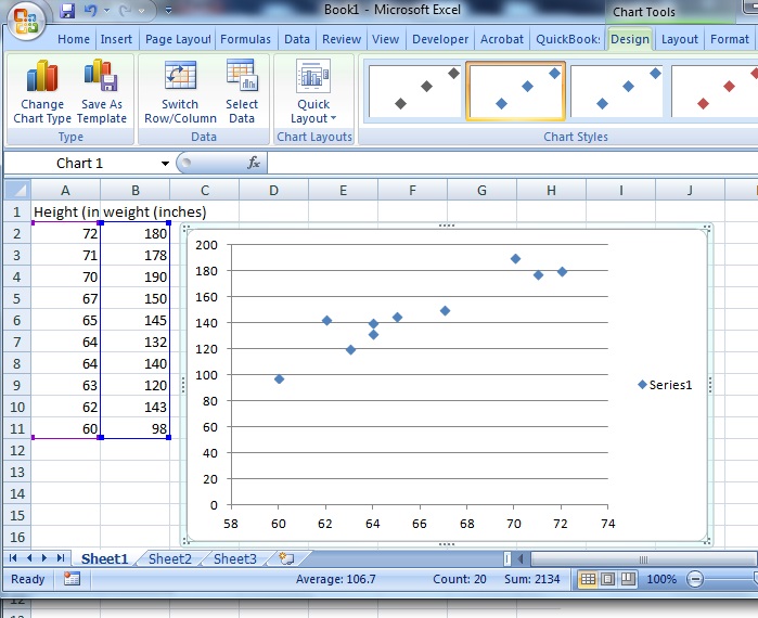
How to Create a Scatterplot Matrix in Excel (With Example) Step 2: Create the Scatterplots. Next, let's highlight the cell range A2:B9, then click the Insert tab, then click the Scatter button within the Charts group. The following scatterplot of points vs. assists will automatically be created: Next, perform the following steps: Click on the values on the x-axis and change the minimum axis bound to 80. how to make a scatter plot in Excel — storytelling with data Highlight the two columns you want to include in your scatter plot. Then, go to the " Insert " tab of your Excel menu bar and click on the scatter plot icon in the " Recommended Charts " area of your ribbon. Select "Scatter" from the options in the "Recommended Charts" section of your ribbon. chandoo.org › wp › change-data-labels-in-chartsHow to Change Excel Chart Data Labels to Custom Values? May 05, 2010 · The Chart I have created (type thin line with tick markers) WILL NOT display x axis labels associated with more than 150 rows of data. (Noting 150/4=~ 38 labels initially chart ok, out of 1050/4=~ 263 total months labels in column A.) It does chart all 1050 rows of data values in Y at all times. excel - How to getting text labels to show up in scatter chart - Stack ... How to getting text labels to show up in scatter chart. I want text labels for my scatter plot that is connected with points in the graph. my data is like this. The chart removes the labels and places numbers. How do I get the text labels back?
How to Make a Scatter Plot in Excel | Itechguides.com
How to set multiple series labels at once - Microsoft Tech Community Click anywhere in the chart. On the Chart Design tab of the ribbon, in the Data group, click Select Data. Click in the 'Chart data range' box. Select the range containing both the series names and the series values. Click OK. If this doesn't work, press Ctrl+Z to undo the change. 0 Likes Reply Nathan1123130 replied to Hans Vogelaar
Scatter Plot / Scatter Chart: Definition, Examples, Excel/TI-83/TI-89/SPSS - Statistics How To
How to add text labels on Excel scatter chart axis Stepps to add text labels on Excel scatter chart axis 1. Firstly it is not straightforward. Excel scatter chart does not group data by text. Create a numerical representation for each category like this. By visualizing both numerical columns, it works as suspected. The scatter chart groups data points. 2. Secondly, create two additional columns.
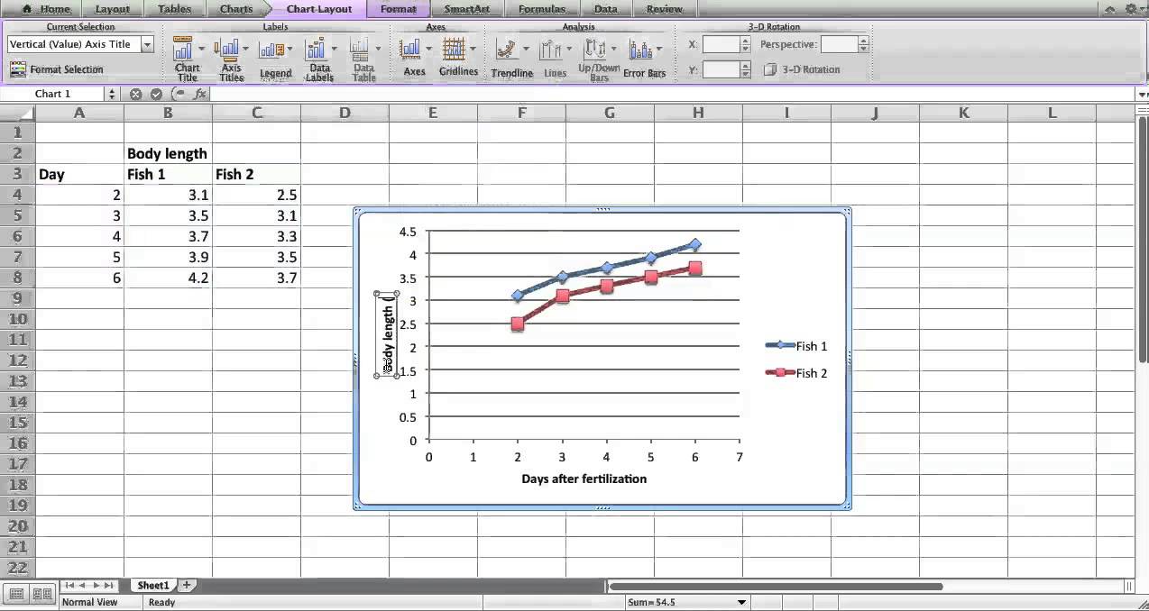
Making a scatter plot in Excel Mac 2011 - YouTube
› documents › excelHow to display text labels in the X-axis of scatter chart in ... Display text labels in X-axis of scatter chart. Actually, there is no way that can display text labels in the X-axis of scatter chart in Excel, but we can create a line chart and make it look like a scatter chart. 1. Select the data you use, and click Insert > Insert Line & Area Chart > Line with Markers to select a line chart. See screenshot:
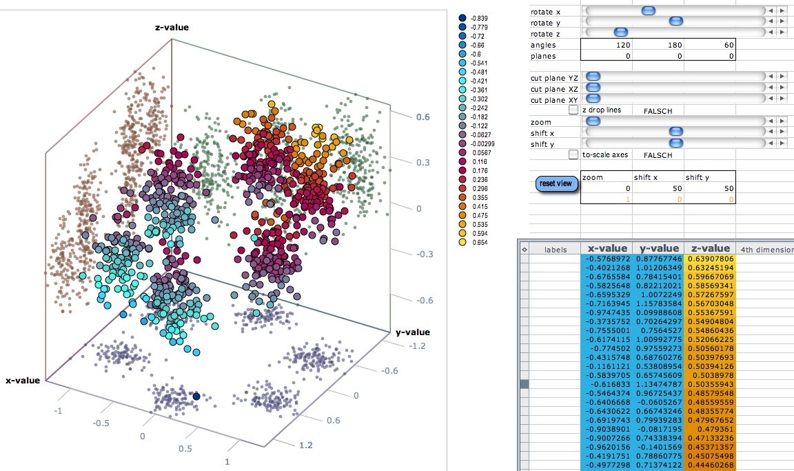
3d scatter plot for MS Excel
How to Add X and Y Axis Labels in Excel (2 Easy Methods) 2. Using Excel Chart Element Button to Add Axis Labels. In this second method, we will add the X and Y axis labels in Excel by Chart Element Button. In this case, we will label both the horizontal and vertical axis at the same time. The steps are: Steps: Firstly, select the graph. Secondly, click on the Chart Elements option and press Axis Titles.
Scatter Chart in Excel (Examples) | How To Create Scatter Chart in Excel?
support.microsoft.com › en-us › topicPresent your data in a scatter chart or a line chart Scatter charts and line charts look very similar, especially when a scatter chart is displayed with connecting lines. However, the way each of these chart types plots data along the horizontal axis (also known as the x-axis) and the vertical axis (also known as the y-axis) is very different.

Excel: labels on a scatter chart, read from array - Stack Overflow
Modifying Axis Scale Labels (Microsoft Excel) - tips Follow these steps: Create your chart as you normally would. Double-click the axis you want to scale. You should see the Format Axis dialog box. (If double-clicking doesn't work, right-click the axis and choose Format Axis from the resulting Context menu.) Make sure the Number tab is displayed. (See Figure 1.)
Scatter Chart in Excel (Examples) | How To Create Scatter Chart in Excel?
How to Create a Timeline with Dates in Excel (4 Easy Ways) Select Axis Titles and deselect Gridlines. Then, select Legend >> Right. Next, change the titles and make the graph more understandable. One more time, click on the plus (+) icon and select Data Labels > Left. Now, click on a starting date point and right-clickon it. A menu will occur. Select Format Data Labels from there.

Add Labels to Outliers in Excel Scatter Charts – System Secrets
Scatter Chart Format Labels from Multiple Cells [SOLVED] Re: Scatter Chart Format Labels from Multiple Cells The attached example uses to helper columns to build new data label text first combines the x and y value to get unique values. then test for first occurrence of a unique value and use FILTER and TEXTJOIN to create new text Attached Files 1369379.xlsx (40.1 KB, 1 views) Download Cheers Andy
:max_bytes(150000):strip_icc()/Insert-Chart-XYScatter-1211a3293e86437b86d3ef03f225c39e.jpg)
How to Create a Scatter Plot in Excel
› excel-chart-verticalExcel Chart Vertical Axis Text Labels • My Online Training Hub Apr 14, 2015 · Note how the vertical axis has 0 to 5, this is because I've used these values to map to the text axis labels as you can see in the Excel workbook if you've downloaded it. Step 2: Sneaky Bar Chart. Now comes the Sneaky Bar Chart; we know that a bar chart has text labels on the vertical axis like this:
charts - Plot 2d graph in Excel - Super User
How to Build Excel Panel Chart Trellis Chart Step by Step Panel Chart Steps. The instructions for making a panel chart in Microsoft Excel might look long, and a bit complicated, but I've grouped the instructions into the following 6 main steps: Step 1 -- Add a Separator Field. Step 2 -- Summarize the data. Step 3 -- Copy the pivot table data.

30 Label Scatter Plot Excel - Labels Design Ideas 2020
How to Make a Scatter Plot in Excel with Multiple Data Sets? Press ok and you will create a scatter plot in excel. In the chart title, you can type fintech survey. Now, select the graph and go to Select Data from the Chart Design tools. You can also go to Select Data by right-clicking on the graph. You will get a dialogue box, go to Edit. You will get another dialogue box, in that box for the Series Name ...
31 Label Scatter Plot Excel - Label Design Ideas 2020
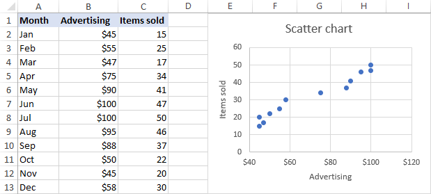
How to make a scatter plot in Excel - Ablebits.com Add labels to scatter plot data points When creating a scatter graph with a relatively small number of data points, you may wish to label the points by name to make your visual better understandable. Here's how you can do this: Select the plot and click the Chart Elements button.
Add Labels to Outliers in Excel Scatter Charts – System Secrets
Excel create scatterplot by categorical variable - Stack Overflow 1. Not sure if there is a better way to do this in Excel but you need to resume your data using a Pivot Table, and then copy/paste the output as range somewhere else and then do your scatterplot (You can't do an scatterplot directly taking a Pivot Table as a source): The setup of my Pivot Table is: Field X to rows section.

Scatter Plot in Excel | How to Create Scatter Chart in Excel?
How to Add Axis Titles in a Microsoft Excel Chart - How-To Geek Click the Add Chart Element drop-down arrow and move your cursor to Axis Titles. In the pop-out menu, select "Primary Horizontal," "Primary Vertical," or both. If you're using Excel on Windows, you can also use the Chart Elements icon on the right of the chart. Check the box for Axis Titles, click the arrow to the right, then check ...
Чарты Excel - Краткое руководство - CoderLessons.com
How to change dot label(when I hover mouse on that dot) of scatter plot To investigate this issue, I made a test using Excel desktop app on my device. As you can see the below screenshot: I am sorry that I don't find any out of box ways to resolve your questions on a scatter plot (chart). But the following thread may help to answer your Expectation: Creating Scatter Plot with Marker Labels - Microsoft Community

Scatter Chart in Excel
How to make a quadrant chart using Excel | Basic Excel Tutorial It is done to ensure all the values and variables are included. To create it, follow these steps 1. Click on an empty cell 2. Go to the Insert tab 3. On the Charts dialog box, select the X Y (Scatter) to display all types of charts. 5. Click Scatter. An empty chart will appear on your worksheet. Add values to the chart. 1.
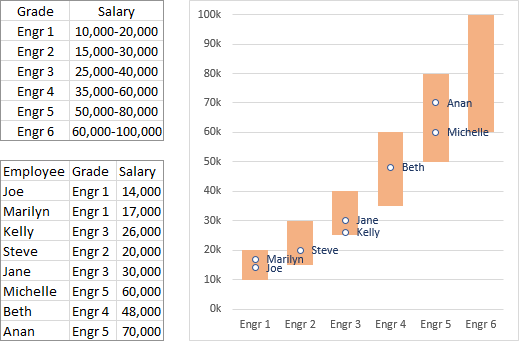
Salary Chart: Plot Markers on Floating Bars - Peltier Tech Blog
Python | Plotting scatter charts in excel sheet using ... - GeeksforGeeks After creating chart objects, insert data in it and lastly, add that chart object in the sheet object. Code #1 : Plot the simple Scatter Chart. For plotting the simple Scatter chart on an excel sheet, use add_chart () method with type 'Scatter' keyword argument of a workbook object. Python3 import xlsxwriter
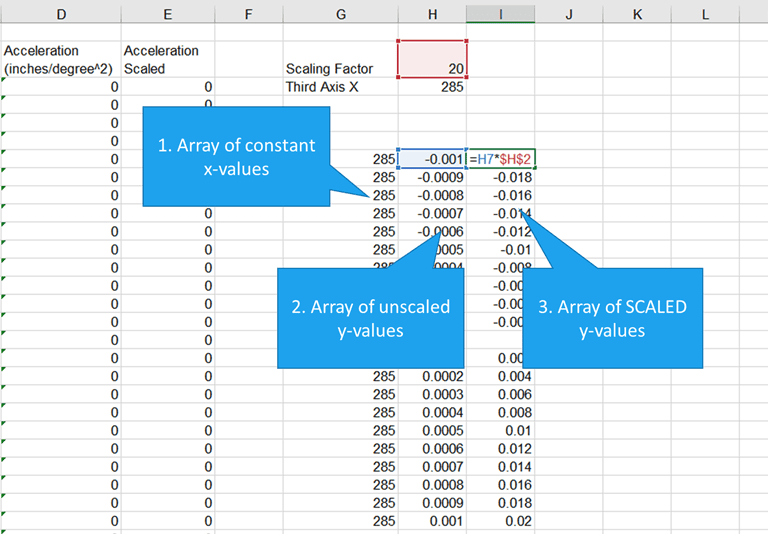
How to Add a Third Y-Axis to a Scatter Chart | EngineerExcel
How to Find, Highlight, and Label a Data Point in Excel Scatter Plot ... By default, the data labels are the y-coordinates. Step 3: Right-click on any of the data labels. A drop-down appears. Click on the Format Data Labels… option. Step 4: Format Data Labels dialogue box appears. Under the Label Options, check the box Value from Cells . Step 5: Data Label Range dialogue-box appears.
Post a Comment for "42 excel scatter chart labels"