38 display data labels excel
Treemap Excel Charts: The Perfect Tool for Displaying Hierarchical Data Go to the INSERT tab in the Ribbon and click on the Treemap Chart icon to see the available chart types. At the time of writing this article, there are 2 options: Treemap and Sunburst. Click the Treemap chart of your choice to add it chart. Clicking the icon inserts the default version of the chart. Now, let's take a look at customization ... Custom Chart Data Labels In Excel With Formulas - How To Excel At Excel Follow the steps below to create the custom data labels. Select the chart label you want to change. In the formula-bar hit = (equals), select the cell reference containing your chart label's data. In this case, the first label is in cell E2. Finally, repeat for all your chart laebls.
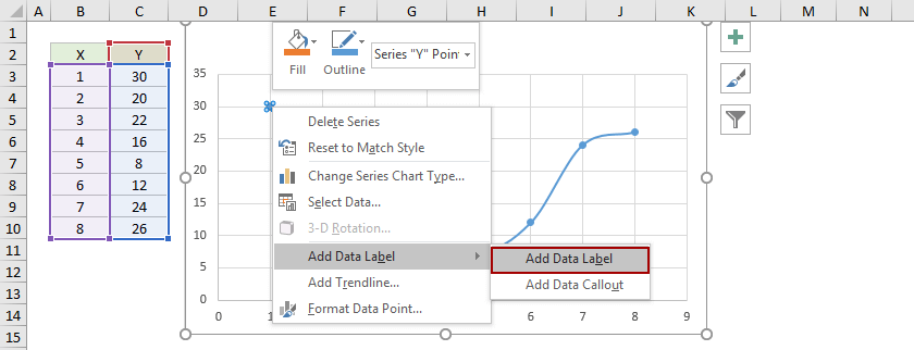
How to add data labels from different column in an Excel chart? This method will introduce a solution to add all data labels from a different column in an Excel chart at the same time. Please do as follows: 1. Right click the data series in the chart, and select Add Data Labels > Add Data Labels from the context menu to add data labels. 2.

Display data labels excel
Adding Data Labels to Your Chart (Microsoft Excel) - ExcelTips (ribbon) Select the position that best fits where you want your labels to appear. To add data labels in Excel 2013 or later versions, follow these steps: Activate the chart by clicking on it, if necessary. Make sure the Design tab of the ribbon is displayed. (This will appear when the chart is selected.) Click the Add Chart Element drop-down list. How to Add Data Labels to an Excel 2010 Chart - dummies On the Chart Tools Layout tab, click Data Labels→More Data Label Options. The Format Data Labels dialog box appears. You can use the options on the Label Options, Number, Fill, Border Color, Border Styles, Shadow, Glow and Soft Edges, 3-D Format, and Alignment tabs to customize the appearance and position of the data labels. How to display text labels in the X-axis of scatter chart in Excel? Display text labels in X-axis of scatter chart. Actually, there is no way that can display text labels in the X-axis of scatter chart in Excel, but we can create a line chart and make it look like a scatter chart. 1. Select the data you use, and click Insert > Insert Line & Area Chart > Line with Markers to select a line chart. See screenshot:
Display data labels excel. How To Plot X Vs Y Data Points In Excel | Excelchat In this tutorial, we will learn how to plot the X vs. Y plots, add axis labels, data labels, and many other useful tips. Figure 1 – How to plot data points in excel. Excel Plot X vs Y. We will set up a data table in Column A and B and then using the Scatter chart; we will display, modify, and format our X and Y plots. Add data labels and callouts to charts in Excel 365 - EasyTweaks.com Step #1: After generating the chart in Excel, right-click anywhere within the chart and select Add labels . Note that you can also select the very handy option of Adding data Callouts. Step #2: When you select the "Add Labels" option, all the different portions of the chart will automatically take on the corresponding values in the table ... to display top 5 data labels on graph [SOLVED] The new table is what your new data series needs to be based on in the graph. What I'm trying to do is make the new data table align perfectly with the existing graph, so that you can add data labels to that data series. This way, your five highest months will always get called out on the graph. Attached Files Excel Charts: Creating Custom Data Labels - YouTube In this video I'll show you how to add data labels to a chart in Excel and then change the range that the data labels are linked to. This video covers both W...
Change the format of data labels in a chart To get there, after adding your data labels, select the data label to format, and then click Chart Elements > Data Labels > More Options. To go to the appropriate area, click one of the four icons ( Fill & Line, Effects, Size & Properties ( Layout & Properties in Outlook or Word), or Label Options) shown here. Data Labels - Intervals | MrExcel Message Board Sub DLabels () Dim ch As Chart, i%, s As Series Set ch = ActiveChart For Each s In ch.SeriesCollection ' all series s.ApplyDataLabels For i = 1 To s.DataLabels.Count If i Mod 6 <> 0 Then s.DataLabels (i).Delete Next Next End Sub Click to expand... Hi Worf, thank you so much for this, this worked. Much appreciated. LC Worf Well-known Member How to show data label in "percentage" instead of - Microsoft Community Select Format Data Labels. Select Number in the left column. Select Percentage in the popup options. In the Format code field set the number of decimal places required and click Add. (Or if the table data in in percentage format then you can select Link to source.) Click OK. Regards, OssieMac. Report abuse. How to Add Data Labels in Excel - Excelchat | Excelchat In Excel 2013 and the later versions we need to do the followings; Click anywhere in the chart area to display the Chart Elements button Figure 5. Chart Elements Button Click the Chart Elements button > Select the Data Labels, then click the Arrow to choose the data labels position. Figure 6. How to Add Data Labels in Excel 2013 Figure 7.
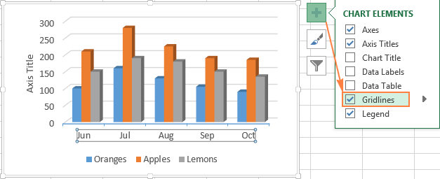
How to Display Percentage in an Excel Graph (3 Methods) Display Percentage in Graph. Select the Helper columns and click on the plus icon. Then go to the More Options via the right arrow beside the Data Labels. Select Chart on the Format Data Labels dialog box. Uncheck the Value option. Check the Value From Cells option. Format Data Labels in Excel- Instructions - TeachUcomp, Inc. Then select the "Format Data Labels…" command from the pop-up menu that appears to format data labels in Excel. Using either method then displays the "Format Data Labels" task pane at the right side of the screen. Set the values and positioning of the data labels in the "Label Options" category, which is shown by default. Excel tutorial: How to use data labels Generally, the easiest way to show data labels to use the chart elements menu. When you check the box, you'll see data labels appear in the chart. If you have more than one data series, you can select a series first, then turn on data labels for that series only. You can even select a single bar, and show just one data label. 10 spiffy new ways to show data with Excel | Computerworld 10 spiffy new ways to show data with Excel ... Right-click the X-axis labels and click Format Axis. In the Axis Options pane, click the Number item and, in Category, select Date from the drop-down ...
How to Make Pie Chart with Labels both Inside and Outside ...
Displaying Large Numbers in K (thousands) or M (millions) in Excel How To Display Numbers in Millions in Excel Right-Click any number you want to convert. Go to Format Cells. In the pop-up window, move to Custom formatting. If you want to show the numbers in Millions, simply change the format from General to 0,,"M" . The figures will now be 23M.
Add or remove data labels in a chart
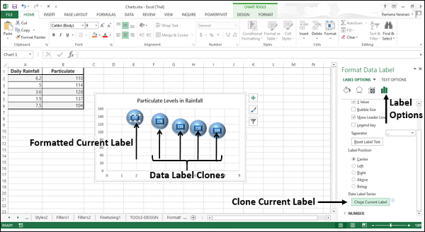
Excel Data Analysis - Data Visualization - tutorialspoint.com Data Labels. Excel 2013 and later versions provide you with various options to display Data Labels. You can choose one Data Label, format it as you like, and then use Clone Current Label to copy the formatting to the rest of the Data Labels in the chart. The Data Labels in a chart can have effects, varying shapes and sizes.
Directly Labeling Excel Charts - PolicyViz
Edit titles or data labels in a chart - support.microsoft.com You can also place data labels in a standard position relative to their data markers. Depending on the chart type, you can choose from a variety of positioning options. On a chart, do one of the following: To reposition all data labels for an entire data series, click a …

How-to Use Data Labels from a Range in an Excel Chart - Excel ...
Data labels not displaying when chart is pasted into PowerPoint Thank you for posting your query in Microsoft Office Community. Before we proceed, I need more information to assist you better. 1) Which options are selected under Add Chart Element > Data labels > More Data label options > Label Options in Excel?

How to add data labels from different column in an Excel chart?
Add or remove data labels in a chart - support.microsoft.com You can add data labels to show the data point values from the Excel sheet in the chart. This step applies to Word for Mac only: On the View menu, click Print Layout. Click the chart, and then click the Chart Design tab. Click Add Chart Element and select Data Labels, and then select a location for the data label option. Note: The options will differ depending on your chart type. If you want ...
![Fixed:] Excel Chart Is Not Showing All Data Labels (2 Solutions)](https://www.exceldemy.com/wp-content/uploads/2022/09/Corrected-Data-Label-Reference-Excel-Chart-Not-Showing-All-Data-Labels.png)
Fixed:] Excel Chart Is Not Showing All Data Labels (2 Solutions)
5 New Charts to Visually Display Data in Excel 2019 - dummies Aug 26, 2021 · Select the data and labels and then click Insert → Maps → Filled Map. Wait a few seconds for the map to load. Resize and format as desired. For example, you could apply one of the chart styles from the Chart Tools Design tab. To add data labels to the chart, choose Chart Tools Design → Add Chart Element → Data Labels → Show. Pouring ...
Excel Chart not showing SOME X-axis labels - Super User
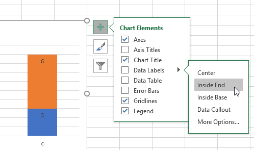
What Are Data Labels in Excel (Uses & Modifications) - ExcelDemy Select Data Labels from the Add Chart Element menu (+) in the top right corner. By clicking the arrow, you can change the position. Select Data Callout if you wish to display your data labels inside a text box. Data labels can be moved inside or outside of data points to make them easier to read.

How to add or move data labels in Excel chart?
How to add data labels in excel to graph or chart (Step-by-Step) 1. Select a data series or a graph. After picking the series, click the data point you want to label. 2. Click Add Chart Element Chart Elements button > Data Labels in the upper right corner, close to the chart. 3. Click the arrow and select an option to modify the location. 4.

Change the format of data labels in a chart
Suppressing Data Labels in Excel if #N/A Value - Stack Overflow The source data consists of formulas which occasionally result in #N/A values. Currently, the data labels for #N/A points are literally displayed as "#N/A". Is there any way I can have Excel suppress the data label altogether if the underlying value is #N/A? If I use =IFERROR (A1,""), then that displays a 0 so that does not work. excel-formula
![Fixed:] Excel Chart Is Not Showing All Data Labels (2 Solutions)](https://www.exceldemy.com/wp-content/uploads/2022/09/Showing-All-Data-Labels-Excel-Chart-Not-Showing-All-Data-Labels.png)
Fixed:] Excel Chart Is Not Showing All Data Labels (2 Solutions)
how to add data labels into Excel graphs - storytelling with data To adjust the number formatting, navigate back to the Format Data Label menu and scroll to the Number section at the bottom. I'll choose Number in the Category drop-down and change Decimal places to 0 (side note: checking the Linked to source box is a good option if you want the labels to reformat when the formatting of the underlying source data changes).

Change the format of data labels in a chart
excel - How to not display labels in pie chart that are 0% - Stack Overflow Generate a new column with the following formula: =IF (B2=0,"",A2) Then right click on the labels and choose "Format Data Labels". Check "Value From Cells", choosing the column with the formula and percentage of the Label Options. Under Label Options -> Number -> Category, choose "Custom". Under Format Code, enter the following:

How to add live total labels to graphs and charts in Excel ...
How to hide zero data labels in chart in Excel? - ExtendOffice 1. Right click at one of the data labels, and select Format Data Labels from the context menu. See screenshot: 2. In the Format Data Labels dialog, Click Number in left pane, then select Custom from the Category list box, and type #"" into the Format Code text box, and click Add button to add it to Type list box. See screenshot: 3.
How to add data labels from different column in an Excel chart?
How to Add Axis Labels in Excel Charts - Step-by-Step (2022) If you want to automate the naming of axis labels, you can create a reference from the axis title to a cell. 1. Left-click the Axis Title once. 2. Write the equal symbol as if you were starting a normal Excel formula. You can see the formula in the formula bar. 3.
Programmatically adding excel data labels in a bar chart ...
How to display text labels in the X-axis of scatter chart in Excel? Display text labels in X-axis of scatter chart. Actually, there is no way that can display text labels in the X-axis of scatter chart in Excel, but we can create a line chart and make it look like a scatter chart. 1. Select the data you use, and click Insert > Insert Line & Area Chart > Line with Markers to select a line chart. See screenshot:

How to show percentages on three different charts in Excel ...
How to Add Data Labels to an Excel 2010 Chart - dummies On the Chart Tools Layout tab, click Data Labels→More Data Label Options. The Format Data Labels dialog box appears. You can use the options on the Label Options, Number, Fill, Border Color, Border Styles, Shadow, Glow and Soft Edges, 3-D Format, and Alignment tabs to customize the appearance and position of the data labels.

How to Change Excel Chart Data Labels to Custom Values?
Adding Data Labels to Your Chart (Microsoft Excel) - ExcelTips (ribbon) Select the position that best fits where you want your labels to appear. To add data labels in Excel 2013 or later versions, follow these steps: Activate the chart by clicking on it, if necessary. Make sure the Design tab of the ribbon is displayed. (This will appear when the chart is selected.) Click the Add Chart Element drop-down list.
Dynamically Label Excel Chart Series Lines • My Online ...

How to use data labels in a chart

axis vs data labels — storytelling with data

Custom data labels in a chart

Apply Custom Data Labels to Charted Points - Peltier Tech

How to add live total labels to graphs and charts in Excel ...
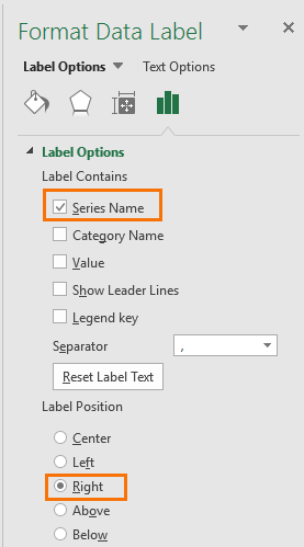
Format Data Label: Label Position - Microsoft Community

How To Show Or Hide Data Labels On MS Excel? | My Windows Hub

Add or remove data labels in a chart
Excel charts: add title, customize chart axis, legend and ...
About Data Labels

Change the format of data labels in a chart

microsoft excel - Adding data label only to the last value ...
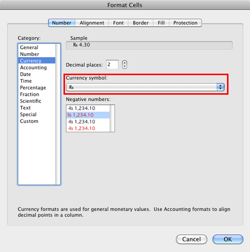
Format Number Options for Chart Data Labels in Excel 2011 for Mac
![Fixed:] Excel Chart Is Not Showing All Data Labels (2 Solutions)](https://www.exceldemy.com/wp-content/uploads/2022/09/Data-Label-Reference-Excel-Chart-Not-Showing-All-Data-Labels.png)
Fixed:] Excel Chart Is Not Showing All Data Labels (2 Solutions)
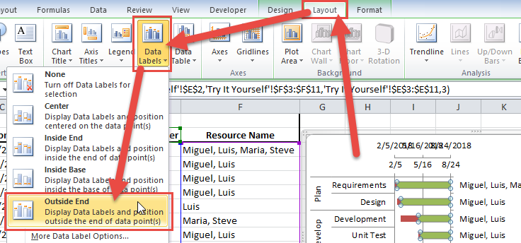
How-to Add Resource Names to Excel Gantt Chart Tasks

Adding rich data labels to charts in Excel 2013 | Microsoft ...
Excel Charts - Aesthetic Data Labels

How to Add Axis Labels to a Chart in Excel | CustomGuide

Dynamically Label Excel Chart Series Lines • My Online ...

Quick Tip: Excel 2013 offers flexible data labels | TechRepublic

Total of chart series – Excel kitchenette
Post a Comment for "38 display data labels excel"